Machine Learning from Scratch

Goal and Purpose

Linear regression is the simplest and arguably most well-known form of machine learning. Linear regression models, as in statistics, are concerned with minimizing error and making the most accurate predictions possible. A neural network can accomplish this by iteratively updating its internal parameters (weights) via a gradient descent algorithm. The Youtube educator 3B1B has a great visualization of gradient descent in the context of machine learning models.

Here, I detail how a simple single-layer model "learns" and how it predicts the outcome of a linear function of the form y=mx+b. This excersize may seem trivial or unecessary ("I can produce a list of solutions for a linear function and plot it with a few lines of code, why do I need a neural network to try and learn how to do the same thing?") but this will act as a backbone to build more complex neural networks for much much more complicated functions.

We will start with the simplest possible neural network, one input neuron and one output neuron with which we will learn how to create linear functions. Then, we will expand upon this simple model by allowing for multidimensional inputs (and thereby allowing for multidimensional outputs as well). Finally, we will complete our foray into Deep Learning by adding "hidden layers" to our neural network. The result will be a modular Deep Learning model that can be easily applied to a diverse set of problems.

The Simplest Neural Network

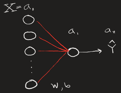
A neural network can be thought of as a function: input, transformation, and output. Therefore, in its most simple representation, a neural network can take a single input, produce an output, and by comparing that output with the known result, can update its internals to better approach the correct output value.

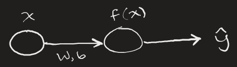
Here, x is some input number, the input is transformed via our neural network function which has parameters W and b (weight and bias). These parameters are subject to change based on how erroneous the network's output ŷ is compared to the actual value we'd expect from input x.

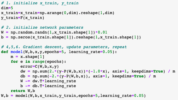
The simple neural network has the following steps:

1. Initialize training input x_train and output y_train. The output here is the expected correct answer.
2. Initialize network parameters W and b . Here the weight array must correspond to the number of inputs. Since we only feed in one input at a time for now, the weights and bias arrays will have shape (1,1). The weight is initialized to a small random number.
3. Define our cost function. The "cost" can be thought of as the error between the expected output and our network's output. "Cost" and "Loss" are similar, though I believe the Loss function is the averaged error when considering a multitude of simultaneous inputs. We'll showcase this later, for now, each error calculation is refered to as the cost.
4. Calculate the components of the gradient of the cost function. In this case: δW/δC and δb/δC.
5. Update the network parameters by reducing by a scaled amount of the gradient components. This is gradient descent.
6. Repeat this process any number of times, called epochs. Return the parameters W and b.
7. Use the model's updated parameters on test data to determine how accurate the trained model is.

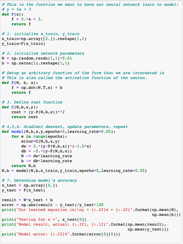
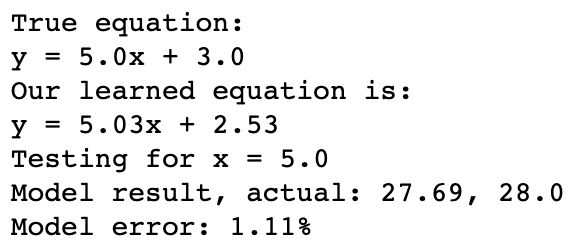
Wonderful! By just feeding our neural network the same number over and over again (5 times in total), we were able to train the network to respond to any other number to within ~1% error.

In Neural Network models, we refer to the weights and biases of the model as the model's parameters. These are elements that change throughout the model's learning process but that we do not necessarily have direct control over. Number of learning iterations (epochs) and the learning rate (which scales by how much parameters W and b are changed) are examples of hyperparameters. We typically DO have direct control over hyperparameters. Below, we can see the effect of a decreased learning rate and increasing epoch number.

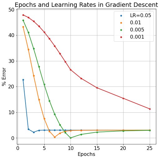
Typically, we'd expect more epoch iterations to lend to less model error since it gives more iterations to improve the model parameters. But this can also have a detrimental effect as the model becomes "over-trained". The learning rate can also be over-tuned, if the learning rate is too large, the model will bounce around it's cost/loss minimum without ever "descending the gradient". If the learning rate is too small, the model will learn very accurately but very slowly, requiring many more epoch iterations to get equivalent results to larger learning rates. As can be seen in the figure below, more epochs can sometimes cause a model's error to rise while smaller learning rates take more epochs to improve.

An Expanding Parameter-Space

An easy way to expand the complexity of our simple neural network (and take another step towards a much more complex deep learning network) is to allow for multi-dimensional inputs. In this case, we can have our model train on 5 values at a time rather than just a single value as before. This can be thought of as training a model to recognize a collection of pixels rather than just a single one, certainly an important progression.

To make compounding improvements, we want to be able to pass multiple inputs into our neural net without having to loop over the input values. We can do this fairly simply by:

1. Establishing our training set as some (1,n) shaped array, with n=5 here. (We can change this later when we add more training examples, think m images with n pixels).
2. Ensuring our parameters W and b reflect the correct dimensions of the incoming multi-dimensional input. Here, those dimensions must be (1,n) since there must be n parameters going to 1 output node.
3. Averaging our gradient calculations for dw and db since our gradient calculation with produce (n,n) matrices for both. We can collapse them to (1,n) arrays and divide by the number of parameters n.

These changes can be seen in the following code snippet (compare to our "simplest" neural network from before). The network output is a little more complicated, as now we now can see the error for each of the n parameters needed for our model to train. In a way, we are training n linear equations at the same time.

The behavior of our models parameters under the shift of the learning rate and epoch number hyperparameters is expectedly improved compared to our "simplest" moedl. Although it's difficult to quantify exactly how this expanded model has improved itself more efficiently, we can certainly see that the model trains to an equally "good" level of low error in less epochs than our previous simple model and that even at the lowest learning rate level our new model can learn more efficiently.

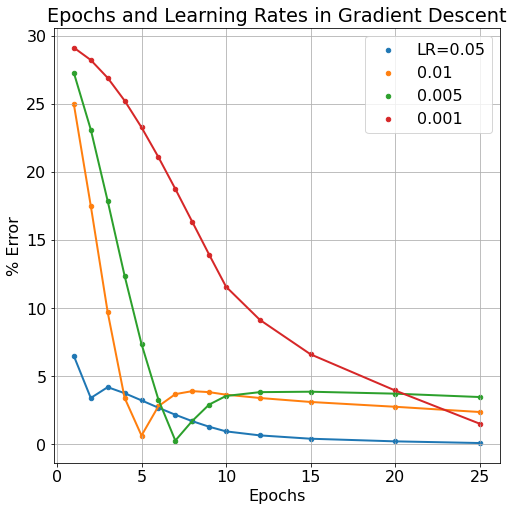
Though we still see similar macro-trends in our new and improved model: it's still possible to over-train the model, and too low of a learning rate can increase the learning iterations needed, thereby requiring undue computational requirements. Next, we'll expand on our neural network once more, this time adding so-called "hidden layers" to the network which will further improve the model's learning capabilities.

Hidden Layers

So far in our machine learning journey we've created "single layer" neural networks and NNs with multipledimensional inputs. In order to unfold this project into the Deep Learning space, we need to be able to create models with so-called "hidden layers". A hidden layer of neurons is not dissimilar to the single output neuron we've seen in our previous model (at least from a functional perspective). Hidden layers can allow a model to better learn more complex functions, a benfit that is amplified with the inclusion of multidimensional hidden layers.

The science behind the optimization of number of hidden layers and their dimensionality is a beyond me at this point but I'm sure I will get to the point of learning more about the inner workings of such models shortly. Now, let's just work on implementing hidden layers, we'll work out the details later.

Backpropagation

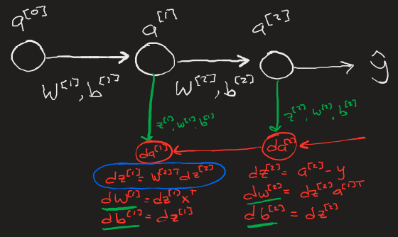
The key mechanism that makes deep learning powerful is Backpropagation which calculates the appropriate changes to all weights and biases in a neural network that will overall reduce the model's cost function.

The simplest representation of backpropagation can be seen here, data from each neuron in each layer during the activation calculation stage is saved in a cache (Z, W, b) to then be used in the backpropagation calculations for the gradients δW, δb.

In Practice

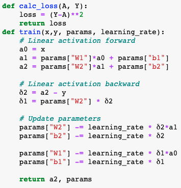
The code for a one hidden layer backpropagation is very simple. It consists of three distinct steps: forward propagation, backwards propagation, and parameter update.

1. Linear activation (forward) - calculate the neuron's activation vlaue with W * x + b for each layer.
2. Linear activation (backward) - calculate the change in the parameters for each neuron (δW = δL/δW, δb = δL/δb) that, when applied to said parameters will lower the models overall loss function.
3. Update parameters - reduce and save the input parameters to be used again in the next iteration.
• W = W-δW\*Ω
• b = b-δb\*Ω

Model Error

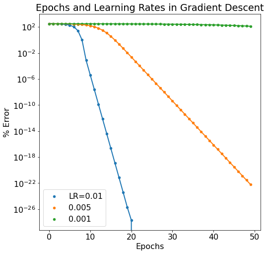
Passing the updated parameters back through the model is an "epoch". As the epoch number increases, we'd expect the error in the model to diminish. We do in fact see this behavior as well as the same dependency on learning rate (lower learning rate makes for a slower learning neural network). Below is a semilogy plot of the same data to reveal the discrepancy between the 0.01 and 0.005 learning rate models.

Next Steps

Next, we need to expand this backpropagation framework to allow for two things. First, we need to be able to add as many hidden layers as we want. Second, we need hidden layers to be modifiable to have any number of neurons. This will result in a fully modular deep learning neural network that can be easily modified on the fly.

What Makes Learning "Deep"?

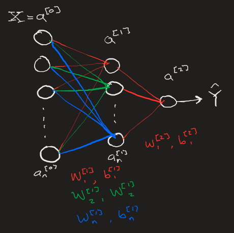
It's important to recognize the profound difference between the models we have built up until now and this current iteration. Previously, we our most advanced model relied on any number of hidden layers consisting of a single node. We found that such a model can still "learn" simple linear functions, but we would not expect a series of linear 1D transformations to be able to model any complex funcitons such as those involved in image recognition.

Expanding each layer into any number of neurons allows for multi-dimensional linear transformations that aid in the extraction of complex patterns within data, decomposing a set of information into otherwise invisible correlations. Once a neural network has the structure necessary to greatly decompose a data set, it becomes much easier for the network to learn from the data, both in time spent learning and the network's ability to accurately respond to new data once the learning is complete.

Coding in the Deep

The code behind coupling high-dimensional neural network layers is surprisingly simple. At its core, transforming activations to a new layer is a linear matrix transformation, one that can be performed quickly and in a single line of code using numpy. The N-dimensional layer can also be built easily with native numpy routines. The most difficult part of this process is the bookkeeping: keeping track of each neuron's weight, bias, and activation as well as the corresponding gradient descent information for the backpropogation step. As a neural network expands, the size of the book to be kept becomes enourmous. Luckily, it's straightforward to build a dictionary to maintain the activation and gradient descent data and ensure that it loops over and includes all data reguardless of any number of layers or number of neurons within individual layers.

def L_layer_model(X, Y, layer_dims, learning_rate=0.05, num_iterations=10, print_cost=False):
    np.random.seed(2)
    costs = []
    # 0. Initialize parameters
    parameters = init_parameters(layer_dims)
    m = Y.shape[1] # used for cost calculation
    
    # 0a. Loop gradient descent
    for i in range(0, num_iterations):
        # 1. Forward Propogation.
        # Get activation of layer L and the cache of intermediate parameters and neuron values.
        caches = []
        A = X
        L = len(parameters) // 2
        for l in range(1,L):
            # Starting from 1 since layer 0 is the input layer.
            A_prev = A
            A, cache = linear_activation_forward(A_prev, parameters['W'+str(l)], parameters['b'+str(l)], 'none') #usually relu
            caches.append(cache)
        # Calling forward activation on last layer separately so we can use sigmoid activation function.
        AL, cache = linear_activation_forward(A, parameters['W'+str(L)], parameters['b'+str(L)], 'none')
        caches.append(cache)

        # 2. Compute Cost
        cost = compute_cost(m, AL, Y)
        cost = np.squeeze(cost) # squeezes out value from weird numpy array format (e.g turns [[17]] to 17).
        costs.append(cost)
        if (print_cost):
            print("Cost is {:.2f} on iteration {}".format(cost, i))
        
        # 3. Backward Propogation: get gradients
        grads = {}

        Y = Y.reshape(AL.shape) # Y and AL are now same shape

        dAL = -2.0*(Y-AL) # Derivative of Loss function with respect to final layer activation AL
        
        # Lth layer (Sigmoid --> Linear) gradients
        current_cache = caches[L-1]
        dA_prev_temp, dW_temp, db_temp = linear_activation_backward(dAL, current_cache, "none") # usually relu
        grads["dA" + str(L-1)] = dA_prev_temp
        grads["dW" + str(L)] = dW_temp
        grads["db"+str(L)] = db_temp
        print(grads)
        
        # Loop from l=L-2 to l=0
        for l in reversed(range(L-1)):
            current_cache = caches[l]
            dA_prev_temp, dW_temp, db_temp = linear_activation_backward(grads["dA"+str(l+1)], current_cache, "none") #usually sigmoid
            grads["dA" + str(l)] = dA_prev_temp
            grads["dW" + str(l + 1)] = dW_temp
            grads["db" + str(l + 1)] = db_temp
            
        # Now have gradients in dictionary grads
        
        # 4. update parameters
        parameters = parameters.copy()
        for l in range(L):
            parameters["W" + str(l+1)] = parameters["W" + str(l + 1)] - learning_rate * grads["dW" + str(l + 1)]
            parameters["b" + str(l + 1)] = parameters["b" + str(l + 1)] - learning_rate * grads["db" + str(l + 1)]
    return parameters, costs

Clearly (or perhaps not), the fundamental steps here are identical to our previous model:

1. Forward propogation - calculate the activation and parameters for each neuron.
2. Caclulate Cost - based on output neuron layer.
3. Backwards propogation - calculating gradient for each neuron and parameter set.
4. update parameters - take a step in the gradient descent of the model.

The significant difference in this iteration of our model is two fold. Firstly, we can treat some neuron layers slightly differently than others. This can be seen in the 3rd parameter of the linear_activation_forward() and linear_activation_backward() functions which takes in a string indicating the type of activation function that we want applied to the neuron activation in the layer. We'll touch on activation functions again soon, but for now our only concern is that unique activation functions require unique forward propogation and backwards gradient calculations. The second major change is how I treat the last layer (index L-1) uniquely and note that usually the activation function here is typically a ReLU. Meanwhile, I treat all other layers (indices 0 to L-2) as having a different activation function, typically a sigmoid, and loop over all of the layers in a single for loop.

Below, notice how I have separate conditionals for the types of activation functions any neuron layer may be receiving.

def init_parameters(layers_dims):
    parameters = {}
    L = len(layers_dims) # number of layers in network
    for l in range(1, L):
        parameters['W'+str(l)] = np.random.randn(layers_dims[l], layers_dims[l-1])*0.01
        parameters['b'+str(l)] = np.zeros((layers_dims[l],1))
    return parameters
def linear_activation_forward(A_prev, W, b, activation):
    Z = np.dot(W, A_prev)+b
    linear_cache = (A_prev, W, b)
    
    if activation == "sigmoid":
        A = 1./(1+np.exp(-1.0*Z))
        activation_cache = (Z)
    
    elif activation == "relu":
        A = np.maximum(0,Z)
        activation_cache = (Z)
    elif activation == "none":
        A = Z
        activation_cache = (Z)
        
    cache = (linear_cache, activation_cache)
    
    return A, cache
def linear_activation_backward(dA, cache, activation):
    linear_cache, activation_cache = cache
    
    # Compute dZ = dA * g'(Z) where g'(Z) is the derivative of the activation function.
    if activation == "relu":
        # Derivative of ReLU
        if activation_cache.any() < 0:
            dZ = 0
        else:
            dZ = dA
    if activation == "sigmoid":
        # Derivative of sigmoid
        dZ = dA * (1./(1+np.exp(-1.0*activation_cache))) * (1 - (1./(1+np.exp(-1.0*activation_cache))))
    if activation =="none":
        dZ = dA
    
    # Get grads of this layer as well as dA for next layer in back prop
    A_prev, W, b = linear_cache
    m = A_prev.shape[1]
    dW = np.dot(dZ, A_prev.T) / m
    db = np.sum(dZ, axis=1, keepdims=True) / m
    dA_prev = np.dot(W.T, dZ)
    
    return dA_prev, dW, db

def compute_cost(m, AL, Y):
    # Simple cost
    #print("AL, Y", AL, Y)
    cost = (Y - AL)**2
    #cost = (-1./m)*np.sum(np.multiply(Y,np.log(AL)) + np.multiply((1-Y), np.log(1-AL)))
    return cost